Retrieval data types
Multiple functions are available to serialize the Topology object. All of them are shown in this table below including the required hard and soft dependencies and further described below.
| Functions | Required Packages |
|---|---|
| topojson.Topology().to_json() | Shapely, NumPy |
| topojson.Topology().to_dict() | Shapely, NumPy |
| topojson.Topology().to_svg() | Shapely, NumPy |
| topojson.Topology().to_geojson() | Shapely, NumPy |
| topojson.Topology().to_alt() | Shapely, NumPy, Altair* |
| topojson.Topology().to_gdf() | Shapely, NumPy, GeoPandas* |
| topojson.Topology().to_widget() | Shapely, NumPy, Altair*, Simplification*, ipywidgets* (+ labextension) |
* optional dependencies
Note: Only the serialization to different output types is described here. See ‘settings and tuning’ for detailed examples of all options regarding creating the Topology object.
.to_json()
Serialize the Topology object into JSON. This is what is called TopoJSON.
Example 🔧
Given the following two polygons:
import topojson as tp
from shapely import geometry

data = [
    {"type": "Polygon", "coordinates": [[[0, 0], [1, 0], [1, 1], [0, 1], [0, 0]]]},
    {"type": "Polygon", "coordinates": [[[1, 0], [2, 0], [2, 1], [1, 1], [1, 0]]]}
]
geometry.GeometryCollection([geometry.shape(g) for g in data])

The Topology can be computed
topo = tp.Topology(data)
And serialized and saved into a JSON (TopoJSON) file:
topo.to_json('my_file.topo.json')
To inspect the JSON object first, leave out the filepath (fp) argument.
print(topo.to_json())
{"type":"Topology","objects":{"data":{"geometries":[{"type":"Polygon","arcs":[[-2,0]]},{"type":"Polygon","arcs":[[1,2]]}],"type":"GeometryCollection"}},"bbox":[0.0,0.0,2.0,1.0],"transform":{"scale":[2.000002000002e-06,1.000001000001e-06],"translate":[0.0,0.0]},"arcs":[[[500000,0],[-500000,0],[0,999999],[500000,0]],[[500000,0],[0,999999]],[[500000,999999],[499999,0],[0,-999999],[-499999,0]]]}
Default is a compact form of JSON. If you like a more readable format, set pretty=True.
print(topo.to_json(pretty=True))
{
    "type": "Topology",
    "objects": {
        "data": {
            "geometries": [
                {"type": "Polygon", "arcs": [[-2, 0]]}, {"type": "Polygon", "arcs": [[1, 2]]}
            ],
            "type": "GeometryCollection"
        }
    },
    "bbox": [0.0, 0.0, 2.0, 1.0],
    "transform": {
        "scale": [2.000002000002e-06, 1.000001000001e-06], "translate": [0.0, 0.0]
    },
    "arcs": [
        [[500000, 0], [-500000, 0], [0, 999999], [500000, 0]], [[500000, 0], [0, 999999]],
        [[500000, 999999], [499999, 0], [0, -999999], [-499999, 0]]
    ]
}
The pretty option depends on the setting indent and maxlinelength, these default to 4 and 88 respectively.
.to_dict()
Serialize the Topology object into a Python Dictionary.
Example 🔧
We use the data as is prepared in the .to_json() section.
topo.to_dict()
{'type': 'Topology',
 'objects': {'data': {'geometries': [{'type': 'Polygon', 'arcs': [[-2, 0]]},
    {'type': 'Polygon', 'arcs': [[1, 2]]}],
   'type': 'GeometryCollection'}},
 'bbox': (0.0, 0.0, 2.0, 1.0),
 'transform': {'scale': [2.000002000002e-06, 1.000001000001e-06],
  'translate': [0.0, 0.0]},
 'arcs': [[[500000, 0], [-500000, 0], [0, 999999], [500000, 0]],
  [[500000, 0], [0, 999999]],
  [[500000, 999999], [499999, 0], [0, -999999], [-499999, 0]]]}
In the computation of the Topology object a few options are adopted. To include these options in the Python Dictionary use options=True.
topo.to_dict(options=True)
{'type': 'Topology',
 'objects': {'data': {'geometries': [{'type': 'Polygon', 'arcs': [[-2, 0]]},
    {'type': 'Polygon', 'arcs': [[1, 2]]}],
   'type': 'GeometryCollection'}},
 'bbox': (0.0, 0.0, 2.0, 1.0),
 'transform': {'scale': [2.000002000002e-06, 1.000001000001e-06],
  'translate': [0.0, 0.0]},
 'arcs': [[[500000, 0], [-500000, 0], [0, 999999], [500000, 0]],
  [[500000, 0], [0, 999999]],
  [[500000, 999999], [499999, 0], [0, -999999], [-499999, 0]]],
 'options': {'topology': True,
  'prequantize': True,
  'topoquantize': False,
  'presimplify': False,
  'toposimplify': False,
  'shared_coords': True,
  'prevent_oversimplify': True,
  'simplify_with': 'shapely',
  'simplify_algorithm': 'dp',
  'winding_order': 'CW_CCW'}}
.to_svg()
Serialize the Topology object into a visual Support Vector Graphic (SVG) mesh.
Example 🔧
We use the data as is prepared in the .to_json() section.
topo.to_svg()
The output is a mesh and information of polygons are not included. To draw each captured linestring separate use separate=True.
topo.to_svg(separate=True)
0 LINESTRING (1.000001000001 0, 0 0, 0 0.9999999999999999, 1.000001000001 0.9999999999999999)1 LINESTRING (1.000001000001 0, 1.000001000001 0.9999999999999999)
2 LINESTRING (1.000001000001 0.9999999999999999, 2 0.9999999999999999, 2 0, 1.000001000001 0)

.to_geojson()
Serialize the Topology object into GeoJSON. This destroys the Topology.
Example 🔧
We use the data as is prepared in the .to_json() section.
Serialize and save into a JSON (GeoJSON) file
topo.to_geojson('my_file.geo.json')
To inspect the JSON object first, leave out the filepath (fp) argument.
print(topo.to_geojson())
{"type":"FeatureCollection","features":[{"id":0,"type":"Feature","geometry":{"type":"Polygon","coordinates":[[[1.000001000001,0.9999999999999999],[0.0,0.9999999999999999],[0.0,0.0],[1.000001000001,0.0],[1.000001000001,0.9999999999999999]]]}},{"id":1,"type":"Feature","geometry":{"type":"Polygon","coordinates":[[[1.000001000001,0.0],[1.9999999999999998,0.0],[1.9999999999999998,0.9999999999999999],[1.000001000001,0.9999999999999999],[1.000001000001,0.0]]]}}]}
Default is a compact form of JSON. If you like a more readable format, set pretty=True.
print(topo.to_json(pretty=True))
{
    "type": "FeatureCollection",
    "features": [
        {
            "id": 0,
            "type": "Feature",
            "geometry": {
                "type": "Polygon",
                "coordinates": [
                    [
                        [1.000001000001, 0.9999999999999999], [0.0, 0.9999999999999999], [0.0, 0.0],
                        [1.000001000001, 0.0], [1.000001000001, 0.9999999999999999]
                    ]
                ]
            }
        },
        {
            "id": 1,
            "type": "Feature",
            "geometry": {
                "type": "Polygon",
                "coordinates": [
                    [
                        [1.000001000001, 0.0], [1.9999999999999998, 0.0],
                        [1.9999999999999998, 0.9999999999999999], [1.000001000001, 0.9999999999999999],
                        [1.000001000001, 0.0]
                    ]
                ]
            }
        }
    ]
}
The pretty option depends on the setting indent and maxlinelength, these default to 4 and 88 respectively.
More options in generating the GeoJSON from the computed Topology are validate (True or False), winding_order and decimals and object_name. Where the TopoJSON standard defines a winding order of clock-wise orientation for outer polygons and counter-clockwise orientation for inner polygons is the winding order in the GeoJSON standard the opposite (CCW_CW). The decimals option defines the number of decimals for the output coordinates. With the option object_name it is possible to specify which object you want to serialize to GeoJSON (in case of multiple objects in the input data), defaults to index 0.
.to_alt()
Serialize the Topology object into an Altair visualization. Altair is an optional dependency and not automatically installed.
Example 🔧
Here we load continental Africa as data file and apply a simplification on the arcs after the topology is computed using toposimplify.
import topojson as tp

import topojson as tp
data = tp.utils.example_data_africa()

topo = tp.Topology(data, toposimplify=4)
Using .to_alt() function one can visualize the Topology using Altair. This means that the TopoJSON as data-object is included in the Vega-Lite specification generated by Altair.
The default will render the Topology as a mesh, meaning that within Vega-Lite the TopoJSON input is rendered as a single unified MultiLineString GeoJSON instance. By default no projection is applied meaning that the input is rendered in a cartesian coordinate system
# this requires the (optional!) package Altair.
topo.to_alt()
A few more convenience options are included for Altair visualizations, such as assigning a color property for individual features and using geographic projections and defining the object_name. With the option object_name it is possible to specify which object you want to serialize to Altair (in case of multiple objects in the input data), defaults to index 0.
Per TopoJSON specification, information of individual features are stored as an nested object within properties. For example here is shown the properties of the feature at index-0:
topo.to_dict()['objects']['data']['geometries'][0]
{'id': '1',
 'type': 'Polygon',
 'properties': {'continent': 'Africa',
  'gdp_md_est': 150600.0,
  'iso_a3': 'TZA',
  'name': 'Tanzania',
  'pop_est': 53950935},
 'bbox': (29.339997592900346,
  -11.720938002166735,
  40.31659000000002,
  -0.9500000000000001),
 'arcs': [[-6, 0, -84, -82, -77, -3, -100, -140, -137]]}
Next, we map the property name of each feature as color property using a nominal (:N) encoding type. The equalEarth is used as geographic projection. By default tooltips are enabled.
# this requires the (optional!) package Altair.
topo.to_alt(color='properties.name:N', projection='equalEarth')
Note: Type encoding needs to be specified and cannot be automatically inferred from TopoJSON input data.
.to_gdf()
Serialize the Topology object into a GeoPandas GeoDataFrame. This destroys the Topology. GeoPandas is an optional dependency and not automatically installed. With the option object_name it is possible to specify which object you want to serialize into a GeoDataFrame using the object_name (in case of multiple objects in the input data), defaults to index 0.
Note: There is no winding-order enforcement in the OGR model; so the Fiona/OGR TopoJSON driver is NOT used in this routine, but the .to_geojson() function.
Example 🔧
Given the included example data set of continental Africa and application of the Topology
import topojson as tp
data = tp.utils.example_data_africa()
topo = tp.Topology(data)
# this requires the (optional!) package GeoPandas.
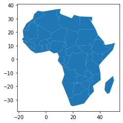
topo.to_gdf().head(3)
topo.to_gdf().plot()
| geometry | id | continent | gdp_md_est | iso_a3 | name | pop_est | |
|---|---|---|---|---|---|---|---|
| 0 | POLYGON ((33.90369435653969 -0.950000999735223… | 1 | Africa | 150600.0 | TZA | Tanzania | 53950935 |
| 1 | POLYGON ((-8.665609889661543 27.65643955148528… | 2 | Africa | 906.5 | ESH | W. Sahara | 603253 |
| 2 | POLYGON ((29.34002323977533 -4.500005567863123… | 11 | Africa | 66010.0 | COD | Dem. Rep. Congo | 83301151 |
.to_widget()
Serialize the Topology object into an interactive IPython Widget. This requires the optional packages simplification, altair and ipywidget(+lab extension). These are not installed automatically.
Example 🔧
Given the included example data set of continental Africa, one can enable the interactive IPython Widget as follow
import topojson as tp

data = tp.utils.example_data_africa()

topo = tp.Topology(data, prevent_oversimplify=False)

# this requires the (optional!) packages: simplification, altair & ipywidget(+labextension).
topo.to_widget()
Note: prevent_oversimplify is set to False since the Douglas-Peucker algorithm within simplification can not prevent oversimplification.
Custom slider options can be set using the slider_toposimplify and slider_topoquantize parameter settings.