Engaging geovisualisations with Vega-Altair
Vega-Altair is a powerful toolkit for creating interactive and engaging geovisualisations in Python.
Lets talk about it.
By Mattijn van Hoek
- PhD on Drought Monitoring from Space & MSc in Geographical Information Management
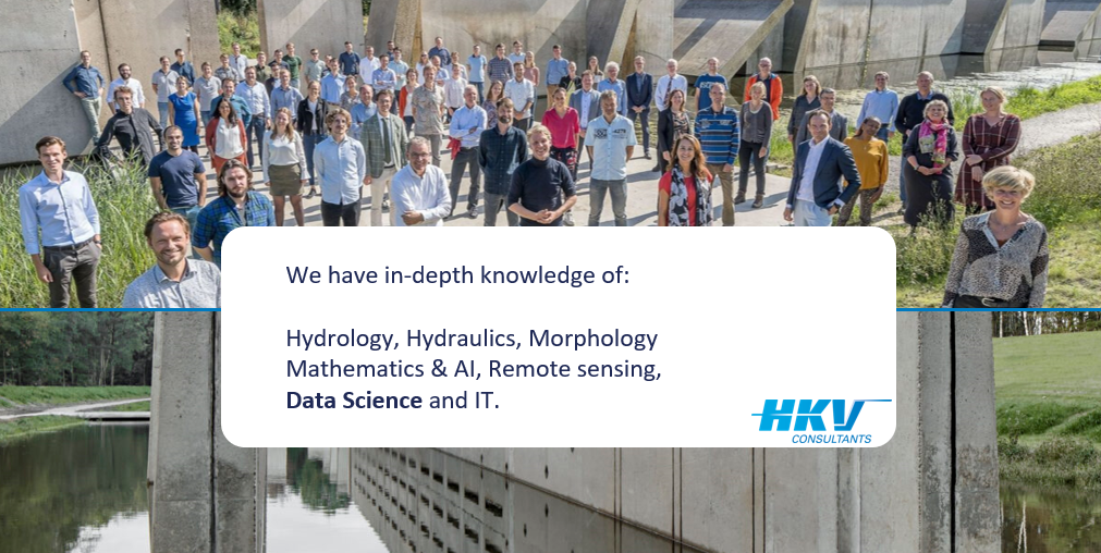
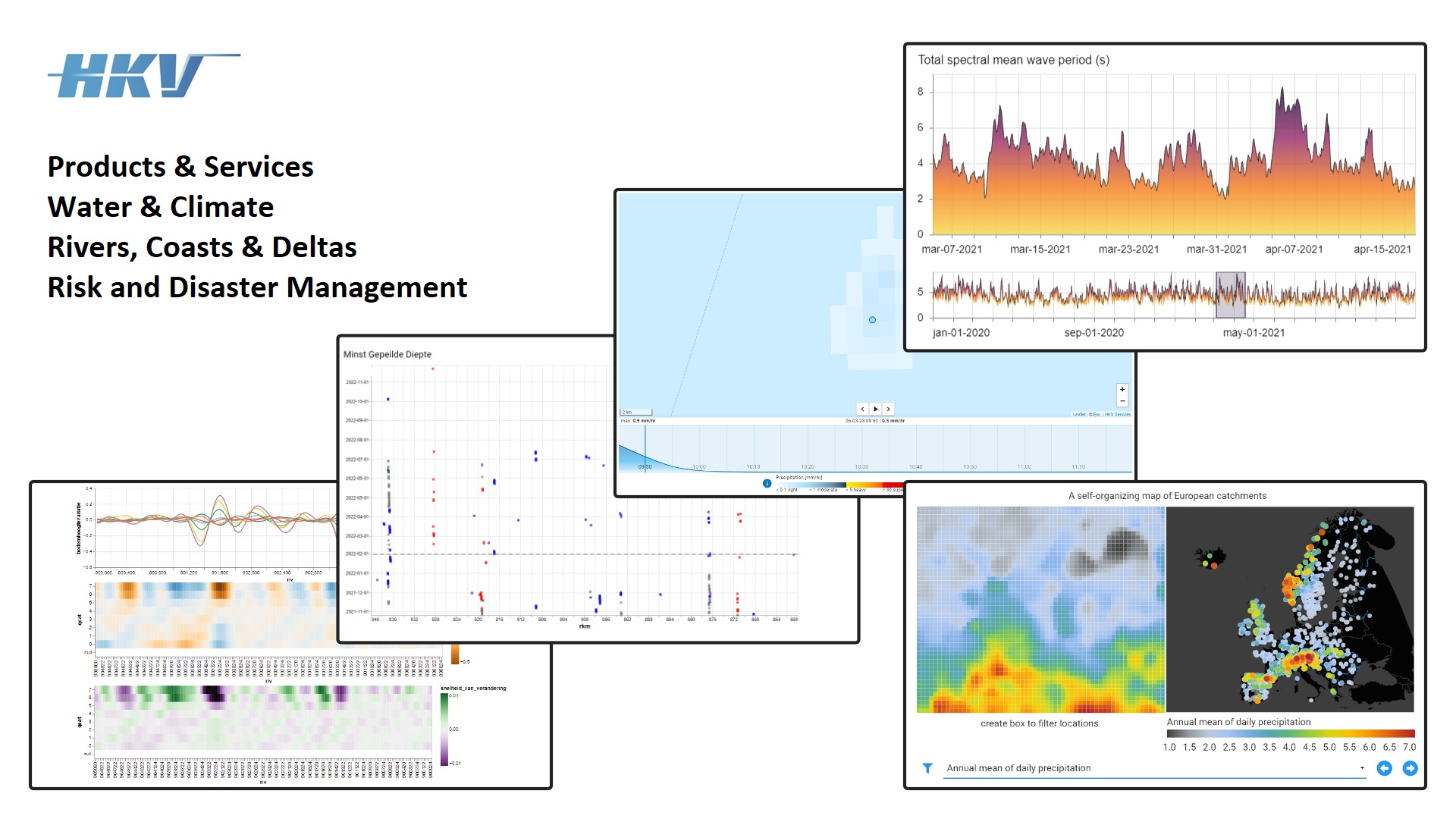
- Senior consultant Product & Services @ HKV Consultants, The Netherlands
- Knowledge entrepreneurs in flood risk and water resources management
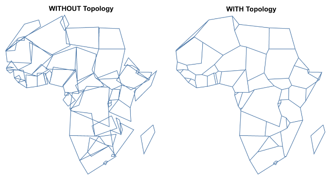
Encode spatial data as topology in Python! 🌍 https://mattijn.github.io/topojson
pip/conda install topojson

VegaFusion: Serverside Scaling for Vega, Started by Jon Mease in 2021
Vega-Altair: Declarative Visualization in Python. Started by Jake Vanderplas & Brian Granger in 2015
Vega-Lite: A Grammar of Interactive Graphics. Started by Arvind Satyanarayan, Kanit Wongsuphasawat, Dominik Moritz in 2014
Vega: A Visualization Grammar. Started by Jeffrey Heer and Arvind Satyanarayan in 2014
D3: Data-Driven Documents, Started by Mike Bostock, Jason Davies, Jeffrey Heer, Vadim Ogievetsky in 2011 | Philippe Rivière (D3-Geo)
For Vega-Altair I also like to mention: Christopher Davis, Joel Östblom, Stefan Binder, Eitan Lees, Ben Welsh (and myself)
NEW! website: https://altair-viz.github.io/
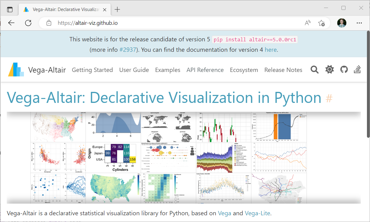
Vega-Altair is a declarative statistical visualization library for Python, based on Vega-Lite.
With Vega-Altair, you can spend more time understanding your data and its meaning. Altair’s API is simple, friendly and consistent and built on top of the powerful Vega-Lite visualization grammar.
This elegant simplicity produces beautiful and effective visualizations with a minimal amount of code.
Monthly PyPi downloads: 10.3M (comparison matplotlib 31.4M, plotly 7.7M)
import altair as alt
from vega_datasets import data
source = data.cars()
alt.Chart(source).mark_point().encode(
x='Horsepower',
y='Miles_per_Gallon',
color='Origin',
)
One of the unique features of Vega-Altair, inherited from Vega-Lite, is a declarative grammar of not just visualization, but also interaction.
brush = alt.selection_interval()
points = alt.Chart(source).mark_point().encode(
x='Horsepower',
y='Miles_per_Gallon',
color=alt.condition(brush, 'Origin', alt.value('lightgray'))
).add_params(
brush
)
bars = alt.Chart(source).mark_bar().encode(
y='Origin',
color='Origin',
x='count(Origin)'
).transform_filter(
brush
)
points & bars
Vega-Altair works with many different geographical data formats, including geojson and topojson files and any data format that supports the geo interface protocol (.__geo_interface__)
Often the most convenient input format is a GeoDataFrame.
Here we load the Natural Earth dataset (50m_admin_0_countries)
import geopandas as gpd
gdf_world = gpd.read_file(r'ne_50m_admin_0_countries/ne_50m_admin_0_countries.shp')
gdf_world = gdf_world[['ADMIN', 'POP_EST', 'geometry']]
gdf_world.head()
| ADMIN | POP_EST | geometry | |
|---|---|---|---|
| 0 | Zimbabwe | 14645468.0 | POLYGON ((31.28789 -22.40205, 31.19727 -22.344... |
| 1 | Zambia | 17861030.0 | POLYGON ((30.39609 -15.64307, 30.25068 -15.643... |
| 2 | Yemen | 29161922.0 | MULTIPOLYGON (((53.08564 16.64839, 52.58145 16... |
| 3 | Vietnam | 96462106.0 | MULTIPOLYGON (((104.06396 10.39082, 104.08301 ... |
| 4 | Venezuela | 28515829.0 | MULTIPOLYGON (((-60.82119 9.13838, -60.94141 9... |
Basic Map
mark_geoshape represents an arbitrary shapes whose geometry is determined by specified spatial data.
By default, Altair applies a default blue fill color and uses a default map projection (equalEarth).
import altair as alt
alt.Chart(gdf_world).mark_geoshape()
We can customize the aesthetics of the mark properties (eg. fill) and define a custom map projection
alt.Chart(gdf_world).mark_geoshape(fill='lightgrey').project(type='albers')
Focus & Filtering
Multiple approaches can be used to focus on specific regions of your spatial data.
Here we load an utility fuction to zoom by a bounding box polygon
from utils_geoconf_23 import *
polygon_bbox = utils_extent(minx=1, miny=51, maxx=9, maxy=55)
polygon_bbox
[{'type': 'Polygon',
'coordinates': (((9, 55), (9, 51), (1, 51), (1, 55), (9, 55)),)}]
We set our polygon_bbox to the fit parameter within the project property in combination with clip=True in the mark properties.
alt.Chart(gdf_world).mark_geoshape(clip=True).project(fit=polygon_bbox)
To improve speed it is often better to clip your region of interest from your GeoDataFrame.
gdf_roi = gdf_world.clip([1, 50.6, 9, 55.3])
gdf_roi.head()
| ADMIN | POP_EST | geometry | |
|---|---|---|---|
| 160 | France | 67059887.0 | POLYGON ((1.57076 50.60000, 1.57949 50.73926, ... |
| 96 | Netherlands | 17332850.0 | MULTIPOLYGON (((5.99395 50.75044, 5.89246 50.7... |
| 156 | Germany | 83132799.0 | MULTIPOLYGON (((5.85752 51.03013, 5.86836 51.0... |
| 217 | Belgium | 11484055.0 | POLYGON ((2.52490 51.09712, 2.96016 51.26543, ... |
| 31 | United Kingdom | 66834405.0 | MULTIPOLYGON (((1.00000 51.80094, 1.00000 52.9... |
Mapping Polygons
We can use the color encoding channel to map the visual property of the ADMIN column.
base = alt.Chart(gdf_roi).mark_geoshape().project(type='mercator')
base.encode(color='ADMIN')
The data type Altair applies is automatically inferred from the GeoDataFrame. Here we concatenate two columns with different datatypes
|: horizontal concat charts
base.encode(color='ADMIN') | base.encode(color='POP_EST')
Mapping Lines
Let's load another dataset containing lines
gdf_rivers_eu = gpd.read_file("https://dmws.hkvservices.nl/dataportal/data.asmx/read?database=vega&key=europe_rivers")
gdf_rivers_roi = gdf_rivers_eu.clip([1, 50.6, 9, 55.3])
gdf_rivers_roi
| name_en | geometry | |
|---|---|---|
| 29 | Rhine | LINESTRING (7.22201 50.60000, 7.20362 50.62161... |
| 52 | Waal | LINESTRING (4.98536 51.82371, 4.72543 51.75666... |
| 43 | Nederrijn | LINESTRING (6.03863 51.87218, 5.92246 51.96055... |
| 24 | Lek | LINESTRING (5.33108 51.96298, 5.16132 51.99352... |
By default Altair assumes for mark_geoshape that the mark’s color is used for the fill color instead of the stroke color. This means that if your source data contain (multi)lines, you will have to explicitly define the filled value as False.
chart_rivers_roi = alt.Chart(gdf_rivers_roi).mark_geoshape(
filled=False, stroke='#0E80AC', strokeWidth=2
)
chart_rivers_roi
Layered Charts
Layered charts allow you to overlay two different charts on the same set of mark. Here we combine our country polygons and river lines.
+: layer charts
chart_roi = alt.Chart(gdf_roi).mark_geoshape(
fill='lightgray', stroke='white', strokeWidth=0.5
)
chart_base = chart_roi + chart_rivers_roi
chart_base
Mapping Points
Let's load another dataset containing points
utils_gdf_points
| location | geometry | |
|---|---|---|
| 0 | delfzijl | POINT (6.93000 53.34000) |
| 1 | harlingen | POINT (5.40000 53.18000) |
| 2 | hoekvanholland | POINT (4.06000 52.00000) |
| 3 | vlissingen | POINT (3.55000 51.44000) |
And combine to our chart_base
chart_pts = alt.Chart(utils_gdf_points).mark_geoshape().encode(
fill='location'
)
chart_base + chart_pts
In combination with mark_text for labels
utils_gdf_points["lon"] = utils_gdf_points.geometry.x
utils_gdf_points["lat"] = utils_gdf_points.geometry.y
chart_text = alt.Chart(utils_gdf_points).mark_text(
align='right', dy=-10
).encode(
longitude="lon", latitude="lat", text="location"
)
chart_base + chart_pts + chart_text
Grammar of Interactivity
So far, the grammar of graphics. Lets continue with grammar of interactivity
param_hover_loc = alt.selection_point(
on='mouseover', clear='mouseout'
)
param_click_loc = alt.selection_point(
fields=['location'], value='hoekvanholland'
)
And a defintion of the the condition how the interactivity should behave
[(<condition_hover>, <if_true>), (<condition_click>, <if_true>)], <if_false>
cond_strokeWidth = utils_condition(
[(param_hover_loc, 2), (param_click_loc, 3)], if_false=0
)
cond_stroke = utils_condition(
[(param_hover_loc, 'red'), (param_click_loc, 'cyan')], if_false=None
)
And define a conditon that response to both hover and click
chart_locs = chart_pts.encode(
strokeWidth=cond_strokeWidth, stroke=cond_stroke
).add_params(
param_hover_loc, param_click_loc
)
chart_geoshape = chart_base + chart_locs + chart_text
chart_geoshape
Interaction
Often a map does not come alone, but is used in combination with another chart.
Here we provide an example of an interactive visualization of a rose plot and a geographic map.
utils_df_storms_rose_binned.head()
| sector | count | mean_windspeed | wind_dir | location | |
|---|---|---|---|---|---|
| 0 | 0 | 77 | 23.228312 | 0.0 - 22.5 | hoekvanholland |
| 1 | 1 | 53 | 23.361321 | 22.5 - 45.0 | hoekvanholland |
| 2 | 2 | 33 | 23.001515 | 45.0 - 67.5 | hoekvanholland |
| 3 | 3 | 32 | 23.115000 | 67.5 - 90.0 | hoekvanholland |
| 4 | 4 | 10 | 22.976000 | 90.0 - 112.5 | hoekvanholland |
We will use an arc mark. Arcs are circular and defined by a center point plus angular and radial extents.
alt.Chart(utils_df_storms_rose_binned).mark_arc(tooltip=True).encode(
theta=alt.Theta('wind_dir').sort(field='sector'),
radius=alt.Radius('count'),
fill='mean_windspeed'
).transform_filter(
alt.datum.location == 'vlissingen'
)
We define similar interactive selection parameters as we did to the locations.
param_hover_wind_dir = alt.selection_point(
on='mouseover', clear='mouseout'
)
param_click_wind_dir = alt.selection_point(
fields=['wind_dir'], value='225.0 - 247.5'
)
Our utility function utils_chart_rose() adds context and interactivity to the rose
chart_rose = utils_chart_rose(utils_df_storms_rose_binned,
param_hover_wind_dir, param_click_wind_dir, param_click_loc
)
chart_rose
And we can combine it with our already defined chart_geoshape
|: horizontal concat charts
chart_rose | chart_geoshape
OK, lets finish it up with a some histgrams. First load the data
print('df shape:', utils_df_storms_hist_binned.shape)
utils_df_storms_hist_binned.head()
df shape: (6464, 14)
| fase | fase_end | fase_count | wind_dir | location | windfase | windfase_end | windfase_count | windduur | windduur_end | windduur_count | opzetduur | opzetduur_end | opzetduur_count | |
|---|---|---|---|---|---|---|---|---|---|---|---|---|---|---|
| 0 | -5.0 | -4.8 | 3.0 | 0.0 - 22.5 | hoekvanholland | NaN | NaN | NaN | NaN | NaN | NaN | NaN | NaN | NaN |
| 1 | -4.6 | -4.4 | 1.0 | 0.0 - 22.5 | hoekvanholland | NaN | NaN | NaN | NaN | NaN | NaN | NaN | NaN | NaN |
| 2 | 2.6 | 2.8 | 6.0 | 0.0 - 22.5 | hoekvanholland | NaN | NaN | NaN | NaN | NaN | NaN | NaN | NaN | NaN |
| 3 | 1.0 | 1.2 | 12.0 | 0.0 - 22.5 | hoekvanholland | NaN | NaN | NaN | NaN | NaN | NaN | NaN | NaN | NaN |
| 4 | 1.6 | 1.8 | 7.0 | 0.0 - 22.5 | hoekvanholland | NaN | NaN | NaN | NaN | NaN | NaN | NaN | NaN | NaN |
We apply a double selection filter. One selection based on the location and one selection on the wind direction.
alt.data_transformers.disable_max_rows()
chart_hist = utils_chart_hists(utils_df_storms_hist_binned,
param_click_wind_dir, param_click_loc
)
chart_hist
Combine everything what we have prepared (& : vertical concat charts)
chart_hist & (chart_rose | chart_geoshape)
We can publish these interactive vizualisations 1:1 as a simple website:
To be shared with our clients
I consider the following a scoop
Still imperative now, but how far can push things using the new alt.param() and alt.expr() in Altair v5?
import altair as alt
from vega_datasets import data
source = alt.topo_feature(data.world_110m.url, "countries")
osm_url, otm_url = ('https://tile.openstreetmap.org/', 'https://tile.opentopomap.org/')
select_urls = alt.binding_select(options=[osm_url, otm_url], name='select tile service')
param_urls = alt.param(bind=select_urls, value=osm_url)
param_tx = alt.param(expr="width / 2")
param_ty = alt.param(expr="height / 2")
param_base_tile_size = alt.param(value=256)
range_z = alt.binding_range(min=2, max=13, step=0.05, name="zoom level")
param_z = alt.param(value=2.75, bind=range_z)
range_x = alt.binding_range(min=-180, max=180, step=0.05, name="rotate longitude")
param_x = alt.param(value=-5.9025, bind=range_x)
range_y = alt.binding_range(min=-60, max=60, step=0.05, name="center latitude")
param_y = alt.param(value=52.56, bind=range_y)
param_tile_url = alt.param(expr=f'{param_urls.name}')
param_zoom = alt.param(expr=f"ceil({param_z.name})")
param_tiles_count = alt.param(expr=f"pow(2, {param_zoom.name})")
param_tile_size = alt.param(
expr=f"{param_base_tile_size.name} * pow(2, {param_z.name} - {param_zoom.name})"
)
param_base_point = alt.param(expr=f"invert('projection', [0, 0])")
param_dii = alt.param(
expr=f"({param_base_point.name}[0] + 180) / 360 * {param_tiles_count.name}"
)
param_di = alt.param(expr=f"floor({param_dii.name})")
param_dx = alt.param(
expr=f"round((floor({param_dii.name}) - {param_dii.name}) * {param_tile_size.name})"
)
param_djj = alt.param(
expr=f"(1 - log(tan({param_base_point.name}[1] * PI / 180) + 1 / cos({param_base_point.name}[1] * PI / 180)) / PI) / 2 * {param_tiles_count.name}"
)
param_dj = alt.param(expr=f"floor({param_djj.name})")
param_dy = alt.param(
expr=f"round((floor({param_djj.name})-{param_djj.name}) * {param_tile_size.name})"
)
tile_list = alt.sequence(0, 4, as_="a", name="tile_list")
image_tiles = (
alt.Chart(tile_list)
.mark_image(
width=alt.expr(f"{param_tile_size.name}"),
height=alt.expr(f"{param_tile_size.name}"),
clip=True,
)
.transform_calculate(b=f"sequence(0, 4)")
.transform_flatten(["b"])
.transform_calculate(
url=f"{param_tile_url.name} + {param_zoom.name} + '/' + (datum.a + {param_di.name} + {param_tiles_count.name}) % {param_tiles_count.name} + '/' + ((datum.b + {param_dj.name})) + '.png'",
x=f"(datum.a * {param_tile_size.name} + {param_dx.name}) + ({param_tile_size.name} / 2)",
y=f"(datum.b * {param_tile_size.name} + {param_dy.name}) + ({param_tile_size.name} / 2)",
)
.encode(
x=alt.X("x:Q").scale(None), y=alt.Y("y:Q").scale(None), url=alt.Url("url:N")
)
)
geoshape_countries = (
alt.Chart(source, width=400, height=400)
.mark_geoshape(
stroke="orange",
strokeWidth=2,
fillOpacity=0.1
)
.encode(fill="id:Q")
.project(
type="mercator",
scale=alt.expr(
f"{param_base_tile_size.name} * pow(2, {param_z.name}) / (2 * PI)"
),
rotate=alt.expr(f"[{param_x.name}, 0, 0]"),
center=alt.expr(f"[0, {param_y.name}]"),
translate=alt.expr(f"[{param_tx.name}, {param_ty.name}]"),
)
)
text_attrib = alt.Chart().mark_text(
text='(C) OpenStreetMap contributors',
dx=-85,
dy=-10
).encode(
x=alt.value(alt.expr('width')),
y=alt.value(alt.expr('height'))
)
chart_inc_tiles = alt.layer(
image_tiles,
geoshape_countries,
text_attrib
).add_params(
param_urls,
param_tile_url,
param_zoom,
param_tiles_count,
param_tile_size,
param_base_point,
param_dii,
param_di,
param_dx,
param_djj,
param_dj,
param_dy,
param_y,
param_x,
param_z,
param_tx,
param_ty,
param_base_tile_size,
)
hopefully one day possible through mark_geoshape(tiles=True)
chart_inc_tiles
What else will be new in Altair 5 (5.0.0rc1 released last week)
The primary change in this release of Altair is the introduction of parameters. There are two types of parameters, selection parameters and variable parameters.
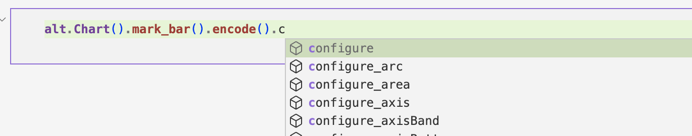
Support for method-based-syntax:
Before only argument-based syntax was possible:
x=alt.X('Horsepower', axis=alt.Axis(tickMinStep=50))Now also method-based syntax:
x=alt.X('Horsepower').axis(tickMinStep=50)
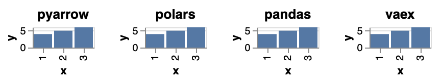
Native Support for DataFrame Interchange Protocol Support (experimental, through
pyarrow)alt.Chart(any_df)
Extensive type hinting
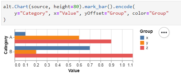
- new
xOffsetandyOffsetencoding channels
Replaced
altair_saverwithvl-convert-pythonfor saving to png/svg (pip-installable, no need for a headless browser anymore)Ordered pandas categorical data are now automatically encoded as sorted ordinal data
selection_interval()support formark_geoshape()
- Docs for spatial data and
mark_geoshapeoptions: